When Fast Ingestion Creates Slow Analytics
Solving the S3 Small-File Problem with Apache Iceberg, Compaction, and Amazon Redshift Spectrum
A reference architecture case study
The Pipeline Was Fast. The Queries Were Slow.
Every metric on the ingestion side looked healthy.
Events from IoT devices, mobile apps, and web clients streamed into an Amazon S3 data lake continuously, durably, with low write latency. The pipeline was doing exactly what it was built to do.
The dashboards built on top of that data told a different story.
Queries that used to return in seconds were taking minutes. Analysts filed tickets. Someone suggested adding more Redshift compute. It didn’t help much.
The two halves of this system were never in conflict about correctness — the data was all there, intact and durable. They were in conflict about shape.
A streaming system optimizes for low-latency, continuous, durable writes.
An analytical engine optimizes for the opposite: fewer, larger, well-organized files it can plan around efficiently.
Nobody had designed for the second half of that sentence, because nothing about the ingestion pipeline was wrong on its own terms.
The problem wasn’t necessarily the amount of data. It was the physical shape of the data.
Architecture Note
This is a reference architecture, not a specific customer engagement.
The workload, file counts, file sizes, and query patterns described below are illustrative and intended to represent a common streaming-ingestion pattern.
Where a claim is backed by AWS or Apache documentation, it is cited. Where a number is illustrative rather than measured, that is stated explicitly.
No benchmark result in this article is presented as measured fact unless independently verified.
1. The Architecture at a Glance
The system has three stages, and the story of this article is what happens to the data’s physical shape as it moves through them.
Ingestion
IoT devices, mobile apps, and web applications emit events continuously.
A streaming layer writes them to an Amazon S3 landing zone as JSON objects, favoring low write latency over downstream analytical concerns.
The Bottleneck
Over hours and days, that landing zone accumulates an enormous number of small JSON objects — illustratively, tens or hundreds of thousands of files averaging around 10 KB each.
Amazon Redshift Spectrum, querying this layout as external tables, absorbs a large and largely avoidable planning and scanning overhead before it ever reaches a useful byte of data.
The Optimization
Apache Iceberg is introduced as a table format and metadata layer over the same S3 storage.
AWS Glue or Spark jobs perform compaction — rewriting many small JSON files into fewer, larger Parquet files — and commit the result as a new Iceberg table snapshot.
Redshift Spectrum then queries a physically consolidated, columnar, metadata-described table instead of a sprawling directory of small text files.
The Architecture in One View
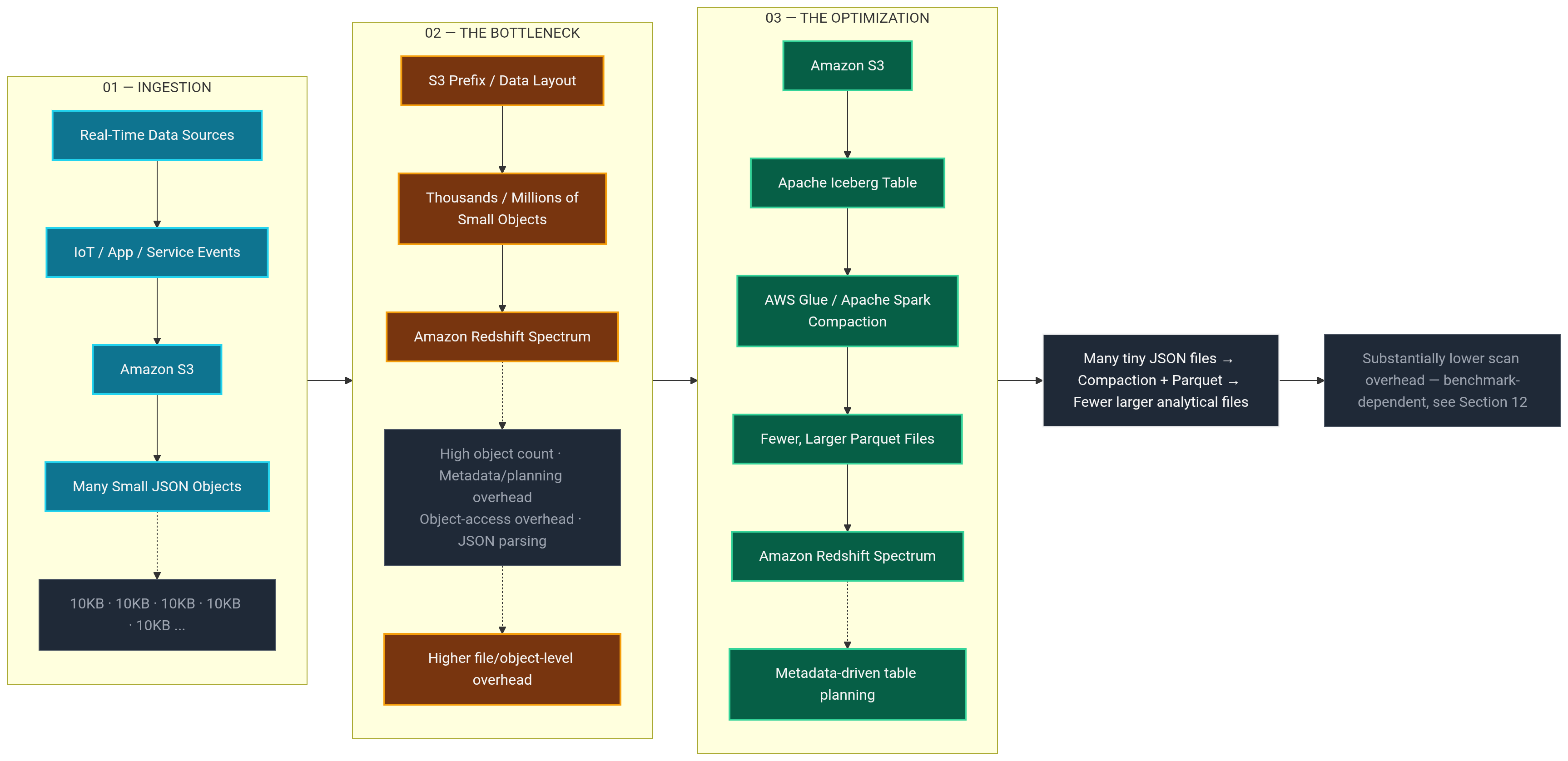
Figure 1 — From fast ingestion to fragmented storage and finally to a metadata-aware, compacted analytical layout.
Three stages, three different concerns:
- how data arrives,
- how data is stored for analysis,
- how a query engine plans and executes against it.
Keeping those three concerns distinct is the throughline of everything that follows.
2. The Incident: Fast Ingestion, Slow Analytics
The presenting symptom was simple:
Dashboard queries against recent event data were getting progressively slower, while the ingestion pipeline showed no degradation at all.
Write throughput was steady.
S3 PUT success rates were normal.
No errors. No backpressure. No obvious infrastructure fault.
That combination — a healthy write path and a degrading read path over the same data — is the signature of a physical layout problem, not necessarily a capacity problem.
If the cluster were simply undersized, you’d expect query performance to be fixable, at least to some degree, by scaling compute.
Here, scaling compute produced only marginal improvement.
That is itself a diagnostic clue worth taking seriously.
Throwing more compute at a query engine doesn’t reduce the number of small objects it has to enumerate, open, and parse before it reaches useful data. It can process some of that overhead in parallel, but only up to a point.
3. The Investigation
The investigation deliberately avoided jumping straight to:
“We need Iceberg.”
It started with measurement.
The team looked at:
- Query latency, broken into planning time and execution time separately, not as one combined number.
- Files scanned per query, compared against the amount of data a query’s predicates should have actually required.
- Bytes scanned, to distinguish “we’re touching too many objects” from “we’re touching too much data.”
- S3 object layout — file count per partition, average object size, and the distribution around that average.
- File format — JSON, uncompressed, record-oriented.
- Partition structure — how data was organized under the landing prefix.
- Query plans — what Redshift Spectrum’s planner was actually doing before scan work began.
This separation matters because file-count reduction and query-latency reduction are not the same claim.
A compaction job can drastically cut the number of files a query touches while only moderately reducing the bytes scanned, particularly for queries that aren’t highly selective.
AWS’s Spectrum performance guidance ties query performance to file size, file format, and partition design as separate, interacting levers — not one lever with one dial.
4. Root Cause #1: The Small-File Explosion
Small files, on their own, aren’t the problem.
A single 10 KB file is nothing.
The problem is what accumulates when a streaming pipeline optimized for write latency runs continuously against the same landing zone for hours and days without any downstream consolidation step.
It’s worth being precise about why a large number of small objects is expensive for an analytical engine.
“More files means more requests, therefore slow” is an oversimplification.
The actual mechanism has several contributing layers:
- Object and file enumeration. Before any scanning happens, the query engine has to discover which objects exist under the relevant prefixes or partitions.
- Metadata discovery and planning overhead. Building an execution plan against a directory structure with an extremely high object count takes measurably longer than planning against a smaller number of well-described files.
- Object access overhead. Each object that participates in a scan carries its own fixed cost — opening it, reading whatever header or footer metadata the format requires, and closing it — independent of how much useful data it contains.
- Task scheduling. A distributed query engine has to schedule work across many small units instead of fewer, larger, more efficient ones, and scheduling overhead doesn’t scale to zero.
- Parsing cost. Record-oriented text formats like JSON have to be parsed row by row, with no ability to skip irrelevant fields during the read.
- Reduced parallelism efficiency. Extremely small files can create more scheduling overhead than benefit, because the fixed cost per file competes with the actual work being done.
The governing principle is:
The smaller the object, the larger the fixed overhead becomes relative to the amount of useful data it contains.
At 10 KB per object and tens of thousands of objects, an analytical engine can spend a disproportionate share of total query time on overhead that has nothing to do with the actual predicates in the query.
S3 Isn’t the Bottleneck
It’s also worth being explicit about what isn’t the bottleneck here.
Amazon S3 itself is not slow, and it is not inherently poorly suited to storing many small objects.
The bottleneck is the interaction between:
- object granularity,
- file format,
- partitioning,
- metadata,
- and how an analytical query engine has to plan and execute a scan across that layout.
That distinction matters.
“S3 is slow” and “this physical layout is expensive to scan” point to very different fixes.
The Small-File Tax
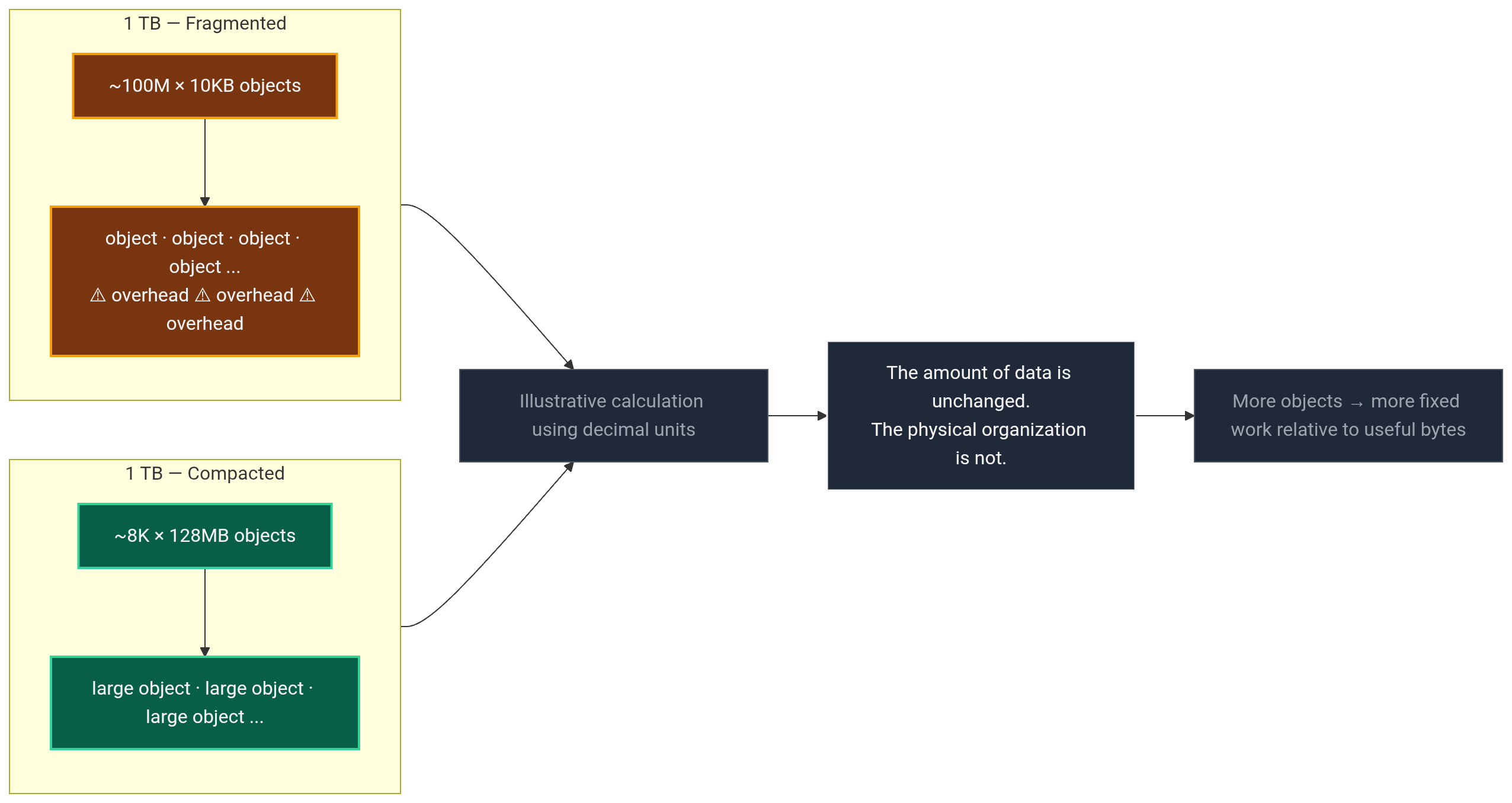
Figure 2 — Illustrative comparison of the same 1 TB dataset represented as many tiny objects versus substantially fewer larger objects.
The important point is not the exact 10 KB or 128 MB figure.
The point is:
The amount of data is unchanged. The physical organization is not.
More objects mean more fixed work relative to useful bytes.
5. Root Cause #2: JSON Is the Wrong Physical Shape for Analytics
JSON is not a bad format.
It’s an excellent format for what it’s usually used for: representing individual records in application and integration contexts where flexibility and human-readability matter more than analytical scan efficiency.
The problem isn’t that JSON is deficient.
It’s that JSON’s design center and an analytical engine’s access pattern point in different directions.
JSON is text-based and record-oriented.
To read any single field from any single record, the parser generally has to read and interpret the whole record.
It isn’t organized around columnar access, which means an analytical query that only needs three columns out of forty still pays the cost of parsing all forty for every record it touches.
It’s important not to overstate this.
JSON isn’t incompressible, and general-purpose compression can and does reduce its size on disk.
But compression on a record-oriented text format doesn’t grant the ability to skip columns during a scan.
That’s where a large share of analytical efficiency actually comes from.
Why Parquet Changes the Equation
Parquet addresses this directly.
It’s columnar, so a query that touches three columns can, subject to how the file was written and how the engine plans the scan, avoid reading data for the other thirty-seven.
It supports efficient compression schemes suited to columnar layouts.
And Parquet files carry embedded statistics — such as min/max values and null counts — that a query engine’s planner can use to skip entire row groups without reading them at all.
The underlying architectural principle is important:
Reducing file count addresses file-level overhead. Moving to a columnar format addresses per-byte scan efficiency.
They are related, additive improvements, not the same improvement described twice.
A workload that fixes file count but stays in JSON still pays the columnar-access penalty.
A workload that moves to Parquet but keeps producing thousands of tiny files still pays the object-overhead penalty.
Both matter independently.
6. Root Cause #3: The Need for Metadata-Aware Table Management
The third root cause is less visible than file size or file format, and it’s the one most often skipped.
Even after you decide to compact files and move to Parquet, someone has to safely manage the process of rewriting a live, continuously growing dataset without:
- breaking readers,
- losing data,
- or leaving the table in an inconsistent state mid-rewrite.
This is a genuinely different problem from:
“What format should the files be?”
or:
“How many files should there be?”
It’s a table-management problem.
How do you:
- track which files currently constitute the authoritative state of a table?
- let a rewrite job replace a large batch of files atomically?
- let readers see a consistent view of the table while compaction is actively running?
A raw S3 prefix with no table format has no native answer to all of these questions.
This is the gap Apache Iceberg is designed to fill.
And it is a distinct concern from file size or file format.
7. The Architectural Intervention
The fix is not:
“Adopt Iceberg.”
It’s the deliberate combination of three things that each solve a different part of the problem.
Apache Iceberg
Provides the table abstraction — the metadata layer that tracks table state, snapshots, and schema, and that makes atomic, consistent rewrites of the underlying files possible.
Parquet
Provides the physical file format — columnar storage, efficient compression, and embedded statistics that a query planner can use.
Compaction
Run as a Spark job on AWS Glue or Amazon EMR, compaction is the process that actually rewrites many small files into fewer, larger ones and commits the result through Iceberg.
Three Technologies. Three Different Jobs.
| Technology / Concept | Primary responsibility |
|---|---|
| Apache Iceberg | Table abstraction, metadata, snapshots, atomic commits |
| Apache Parquet | Physical columnar file format |
| Compaction | Rewrites many smaller files into fewer larger files |
These are three separable technologies performing three separable jobs.
Iceberg is not a file format.
It doesn’t itself make files larger, smaller, columnar, or compressed.
Parquet is not a table format.
It has no concept of snapshots, schema evolution, or atomic multi-file commits on its own.
Compaction is not free.
It is compute work that has to be scheduled, run, monitored, and paid for.
Keeping these boundaries distinct is what separates an accurate explanation of this architecture from a marketing summary of it.
8. How Iceberg Organizes the Table
Iceberg’s contribution is best understood as a metadata hierarchy sitting above the physical Parquet files in S3.
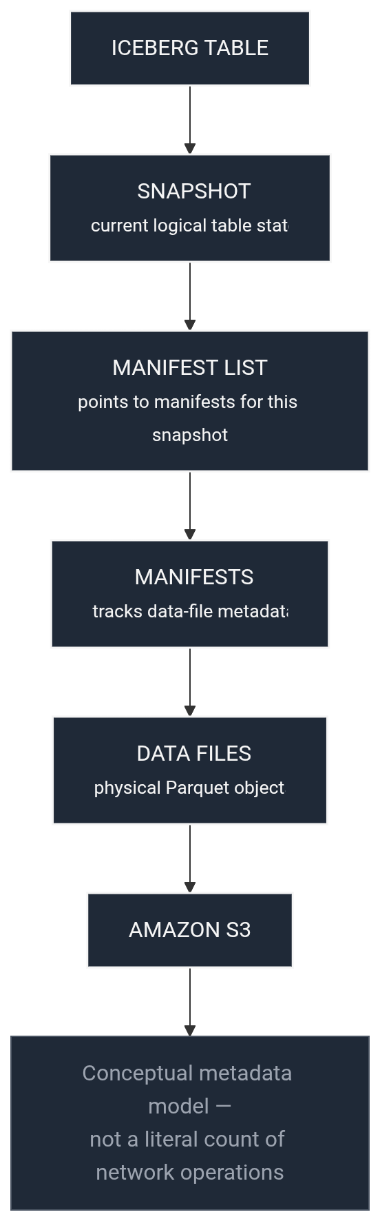
Figure 3 — Conceptual Iceberg metadata hierarchy from table state to physical Parquet objects.
A simplified logical view is:
Iceberg Table
      ↓
Snapshot
      ↓
Manifest List
      ↓
Manifests
      ↓
Data Files
      ↓
Parquet Objects in S3
A snapshot represents the complete, consistent state of the table at a point in time.
Each snapshot points to a manifest list, which in turn references one or more manifests — files that track metadata about groups of data files, including partition values and, when generated, column-level statistics.
The manifests point to the actual data files: the Parquet objects physically stored in S3.
A Necessary Caveat
This hierarchy is a conceptual and logical model for how Iceberg organizes table state and enables metadata-driven planning.
It is not a literal claim about the exact sequence or count of network operations Redshift Spectrum performs for any given query.
What it gives a query engine is the ability to plan from structured metadata about which files are relevant to a query, rather than having to enumerate an entire object listing from S3 directly.
AWS documentation on querying Iceberg tables from Redshift describes this metadata-driven planning model and separately notes that AWS Glue-generated statistics for Iceberg tables can help Redshift’s optimizer reduce the number of files it needs to scan.
Iceberg also provides atomic commits and snapshot isolation.
A compaction job can replace a large batch of small files with a smaller batch of large ones as a single atomic operation.
Readers querying the table mid-rewrite see either the old consistent state or the new one — never a partial, broken mix of both.
That property is what makes it safe to continuously reorganize a live analytical dataset.
And that is a genuinely different contribution from:
“makes files bigger”
or:
“makes queries faster.”
9. How Compaction Changes the Physical Layout
Compaction is the mechanical process that actually does the file rewriting.

Figure 4 — Compaction rewrites physical files while Iceberg manages the resulting table state.
The lifecycle is conceptually:
Small Files
     ↓
Compaction Job
(Glue / Spark)
     ↓
Read Existing Data Files
     ↓
Rewrite / Merge into Larger Parquet Files
     ↓
Atomic Iceberg Commit
     ↓
New Table Snapshot
The job reads a set of existing small files, rewrites their combined contents into a smaller number of larger Parquet files, and commits that rewrite as a new Iceberg snapshot.
The old files aren’t deleted the instant the new ones are written.
They remain part of prior snapshots until retention and expiration policies clean them up.
That is deliberate.
It is what allows time-travel queries and safe rollback if something in the rewrite went wrong.
Compaction Is Recurring
Compaction is recurring, not one-time, because ingestion doesn’t stop.
A landing zone under continuous write load will keep accumulating small files after every compaction run.
That raises an operational question:
How often should compaction actually run?
“Run it daily” is not a universal answer.
The right cadence depends on:
- rate of file accumulation,
- query workload,
- freshness requirements,
- cost of the compaction job,
- partition behavior,
- and available rewrite capacity.
A workload accumulating files faster than a daily job can absorb needs more frequent, threshold-based triggering.
Compact when a partition crosses a file-count or fragmentation threshold rather than on a fixed calendar regardless of actual need.
A workload with a healthy, slowly growing partition doesn’t need the compute cost of a daily rewrite it doesn’t yet require.
10. What Changes at Query Time
With the intervention in place, Redshift Spectrum is querying a table with a materially different physical and metadata profile.
It’s important to state precisely what’s actually happening.
This is exactly the point where oversimplified claims tend to creep in.
Redshift Spectrum does not perform:
“a single metadata lookup”
and then instantly access all relevant data.
That phrase overstates how metadata-driven planning works.
The actual mechanism is a structured, hierarchical process of using Iceberg’s snapshot and manifest metadata to identify a relevant, pruned set of data files before scan work begins.
Nor is it accurate to describe the underlying mechanism as:
“Spectrum issues one HTTP GET request for every file.”
That’s a plausible-sounding simplification, but stating it as a precise fact about Spectrum’s execution path isn’t something the available documentation directly confirms.
The actual overhead mechanism is broader:
- enumeration,
- planning,
- parsing,
- scheduling,
- and object access.
What Can Be Stated with Confidence
Redshift Spectrum performance benefits from:
- columnar file formats,
- appropriately sized files rather than KB-scale objects,
- well-designed partitioning that supports pruning,
- and, specifically for Iceberg tables, Glue-generated statistics that can help the optimizer reduce the number of files it needs to scan.
The architectural change is therefore not:
1 metadata lookup
        ↓
everything is fast
It is:
Fragmented physical layout
        ↓
Metadata-aware table
        ↓
File / partition pruning
        ↓
Fewer, better-organized files
        ↓
More efficient analytical scanning
11. Before vs. After
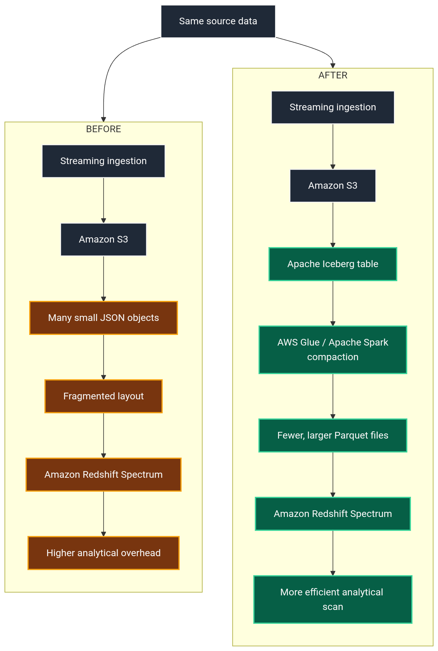
Figure 5 — The ingestion path remains largely unchanged; the downstream analytical representation changes.
Before
Applications (IoT / mobile / web)
     ↓
Streaming ingestion
     ↓
Amazon S3 landing zone
     ↓
Many small JSON objects
(~10 KB, illustrative)
     ↓
Amazon Redshift Spectrum
     ↓
Higher enumeration, planning,
and parsing overhead
After
Applications (IoT / mobile / web)
     ↓
Streaming ingestion
     ↓
Amazon S3 landing zone
     ↓
Apache Iceberg table
     ↓
AWS Glue / Spark compaction
(threshold-based)
     ↓
Fewer, larger Parquet files
committed as new snapshots
     ↓
Amazon Redshift Spectrum
Same Data. Different Physical Layout.
| Aspect | Before | After |
|---|---|---|
| File format | JSON | Parquet |
| Average file size | ~10 KB (illustrative) | 64–128 MB (illustrative target range) |
| File count | Very high | Substantially lower |
| Metadata planning | Directory-level object listing | Iceberg snapshots and manifests |
| Optimizer statistics | Minimal | Glue-generated Iceberg statistics |
| Scan efficiency | Lower — full-record parsing | Higher — columnar, prunable |
| Compression | Text-oriented | Columnar compression |
| Data freshness | Immediate | Slightly delayed, dependent on compaction cadence |
Ingestion behavior is unchanged in this picture.
That’s deliberate.
The applications still write the way they were always going to write.
What changed is entirely downstream, in how that data is subsequently organized for the workload that consumes it.
12. Benchmarking the Improvement
Here is the point where this article deliberately declines to hand you a headline number.
No specific production benchmark result — no percentage, no “Nx faster,” no before/after latency figure — is presented as measured fact in this article because none was independently verified for this reference scenario.
What follows instead is a reproducible methodology, along with hypotheses that AWS’s own documentation supports.
Those hypotheses should be tested against the actual workload before being turned into performance claims.
Benchmark at More Than One Scale
Run the comparison at more than one scale — for example:
- 100 GB
- 1 TB
- 10 TB
Overhead effects at small scale don’t always predict behavior at larger scale.
Variants to Compare
| Variant | Format | Average file size | Table layer |
|---|---|---|---|
| Baseline | JSON | ~10 KB | Raw external table, no Iceberg |
| Optimized — Parquet only | Parquet | 64–128 MB | No Iceberg / minimal metadata |
| Optimized — Parquet + Iceberg | Parquet | 64–128 MB | Iceberg table + Glue-generated statistics |
Including the middle variant matters.
It lets you separate the contribution of file format and file size from the contribution of Iceberg’s metadata layer, rather than crediting one intervention for the combined effect of two.
Representative Query Workload
Test several query shapes:
- time-range filter,
- highly selective predicate,
- aggregation,
- multi-column projection,
- partition-pruned query.
This covers query patterns that can behave differently under fragmented versus consolidated layouts.
Measure the Layers Separately
Measure:
- total query latency,
- planning latency,
- execution latency,
- bytes scanned,
- files scanned,
- observable S3 request patterns where available,
- relevant Spectrum-side query metrics,
- compute consumption,
- cost per query.
Control the Variables
Keep the following identical between runs:
- SQL text,
- Redshift cluster configuration,
- concurrency,
- S3 region,
- partition scheme,
- underlying row content,
- compression settings.
Report More Than a Single Number
Report:
- median,
- p95,
- and the distribution across repeated runs.
Don’t report only the single best-case query.
More importantly, report each metric layer separately rather than collapsing everything into one latency figure.
What the Documentation Supports as a Hypothesis
A reasonable hypothesis is:
- JSON at small file sizes will show the highest planning and scan overhead of the three variants.
- Moving to Parquet will reduce per-byte scan cost through columnar access and compression.
- Adding Iceberg with Glue-generated statistics can further reduce files scanned for selective queries because the optimizer has structured statistics available for pruning.
These are hypotheses to benchmark, not guaranteed results.
If you run this methodology against your own workload and observe a specific speedup — 10x, 50x, 100x, whatever the number turns out to be — that number is a property of:
- your workload,
- your query selectivity,
- your data shape,
- your partitioning,
- your infrastructure,
- and your implementation.
It is not a universal property of Iceberg.
Benchmark the architecture, not the technology label.
13. The Cost of Optimization
It would be dishonest to present this as a pure win.
Compaction is not free.
Pretending otherwise undermines the credibility of everything else in this article.
Costs Introduced
- Glue or Spark compute to run the compaction jobs themselves.
- The rewrite operation’s own I/O — reading the small files being consolidated and writing the new Parquet output.
- Temporary storage overhead during the rewrite.
- Operational complexity: something new to monitor, alert on, and operate.
- A freshness trade-off — data isn’t reflected in the optimized table until it has been through a compaction cycle, so there is an inherent lag between arrival and full analytical optimization.
Costs Potentially Reduced
- Query-side compute spent on unnecessary scanning and parsing.
- The operational and business cost of slow dashboards.
- Reduced request and object-access overhead per query.
The governing economic principle is:
Compaction is worthwhile when the recurring analytical cost and latency caused by a fragmented physical layout exceed the cost of maintaining an optimized one.
For a landing zone that’s rarely queried directly, that calculus might not favor aggressive compaction at all.
For a table backing high-frequency dashboards under continuous analytical load, it usually will.
That’s a workload-specific judgment, not a default answer.
14. Production Guardrails
A physical-layout optimization introduces its own failure modes.
None of these are exotic.
They’re the ordinary operational reality of running compaction as a continuous process against a continuously growing dataset.
| Failure mode | Why it happens | Detection | Mitigation |
|---|---|---|---|
| Compaction lag | Files accumulate faster than compaction jobs can process them | File count and freshness lag trending upward | Threshold-based triggers; sufficient rewrite capacity |
| Compaction storms | Multiple large rewrites trigger simultaneously | Spikes in job concurrency and compute cost | Scheduling controls, rate limiting, partition-scoped optimization |
| Over-partitioning | Partition design is too fine-grained | High file count per partition | Coarser partitioning aligned to actual query patterns |
| Wrong target file size | Files end up too small or too large | File-size distribution tracked against target | Tune thresholds against workload behavior |
| Snapshot accumulation | Old snapshots are retained indefinitely | Snapshot count and age trending upward | Retention and expiration policies |
| Orphaned files | Failed rewrites leave unreferenced objects | Catalog-to-S3 mismatch | Scheduled cleanup / orphan-file removal |
| Failed compaction jobs | Jobs fail without being noticed | Job alerts and freshness monitoring | Retries, backoff, lag-based alerting |
| Raw-zone querying | Consumers bypass the optimized table | Query source auditing | Access controls and catalog separation |
None of these are reasons to avoid the architecture.
They’re the reason it needs monitoring, lifecycle management, and operational ownership rather than being treated as a one-time migration.
15. When You Don’t Actually Need Iceberg
This is worth stating directly because it’s the section most often missing from articles that are ultimately trying to sell a technology rather than solve a problem:
Iceberg is not the first thing to try.
The decision order is roughly in ascending order of complexity.
1. Fix Ingestion Batching or Windowing First
If the root problem is that the producer is flushing far more frequently than necessary, adjusting write batching or windowing at the source can eliminate the small-file problem before it ever reaches S3.
This is the cheapest fix and the one most often skipped in favor of a downstream architectural solution.
2. Write Directly to Parquet
If the dataset is relatively simple, doesn’t need concurrent readers and writers reasoning about consistent snapshots, and doesn’t need to evolve its schema or partitioning over time, writing directly to Parquet may be sufficient.
3. Run Scheduled or Threshold-Based Compaction
Where the operational need is genuinely just:
“Consolidate files periodically.”
you may not need a table format if snapshot isolation, schema evolution, and other table semantics aren’t required.
4. Adopt Iceberg with Compaction
Iceberg becomes compelling when the dataset genuinely needs table abstraction:
- concurrent readers and writers operating safely against an evolving dataset,
- schema evolution,
- partition evolution,
- atomic multi-file commits,
- time travel,
- and long-lived governance over an analytical table’s lifecycle.
The conclusion is not:
“Everyone should use Iceberg.”
It is:
Use the simplest architecture that solves the actual problem.
Introduce a table format when the dataset’s lifecycle actually justifies the complexity it adds.
A batch job that compacts JSON into Parquet on a schedule, with no table format at all, may be entirely sufficient for a dataset that doesn’t need concurrent writers or schema evolution.
Iceberg earns its place when the table’s operational lifecycle demands more than compaction alone can provide.
16. Architecture Decision Framework
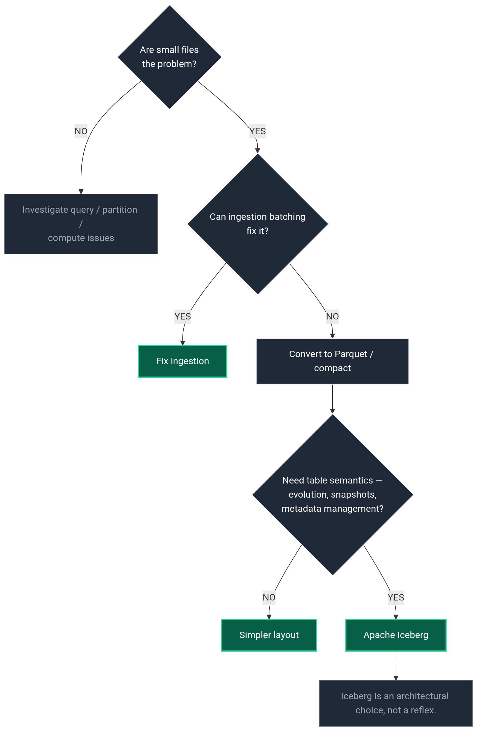
Figure 6 — A decision framework for determining whether the workload actually needs Iceberg.
| Approach | Complexity | Solves Small Files? | Adds Table Semantics? | Best Fit |
|---|---|---|---|---|
| Better ingestion batching | Low | Yes | No | Root cause is upstream write behavior |
| JSON → Parquet | Low–Medium | Partially | No | Simple, relatively static analytical datasets |
| Standalone scheduled / threshold compaction | Medium | Yes | No | Periodic file consolidation without table semantics |
| Iceberg + compaction | Medium–High | Yes | Yes | Evolving datasets requiring table governance |
| Alternative table format | Medium–High | Yes | Yes | Workloads favoring another format’s semantics |
This table isn’t meant to declare a winner.
It’s meant to help you place your own workload against the actual axes that matter:
- How complex is the fix you’re willing to operate?
- Does the dataset genuinely need table-level semantics?
- Or does it simply need a cleaner physical layout?
What This Article Is — and Isn’t
This article presents a reference architecture, not a production benchmark or customer case study.
It is not an argument that every S3 data lake should use Apache Iceberg.
It is not a claim that 128 MB is the universally correct file size.
It is not a guarantee that compaction produces a specific percentage improvement.
It is not a claim that S3 performs poorly when a bucket contains many objects.
And it is not a claim that Redshift Spectrum performs one specific network operation per file as the sole explanation for the small-file problem.
The problem is the interaction between:
file granularity + physical format + partitioning + metadata management + analytical workload
That is the architectural boundary that matters.
17. Conclusion
The problem this article describes was never really that the data lake contained too much data.
It was that the data had been physically organized around the needs of the producer — low-latency, continuous, durable writes — rather than the needs of the analytical consumer, which wants the opposite:
fewer, larger, well-described files it can plan around efficiently.
The fix is not:
“Use Iceberg.”
It’s the deliberate combination of:
- appropriate ingestion behavior,
- an appropriate physical file format,
- sensible file sizing tuned to the actual workload,
- a compaction process that runs on a cadence matched to real accumulation and freshness needs,
- and a metadata-aware table management layer introduced when — and only when — the dataset’s lifecycle actually justifies it.
Design the way data arrives for ingestion.
Design the way data is stored for analytics.
And reach for a table format when the lifecycle of that analytical data genuinely demands one — not because it’s the technology attached to the fastest-sounding benchmark number you’ve seen.
The goal isn’t to make the data lake look modern. The goal is to make the physical data layout fit the workload.
Sources
- Amazon Redshift Spectrum query performance — AWS Documentation
- Data files for queries in Amazon Redshift Spectrum — AWS Documentation
- Using Apache Iceberg tables with Amazon Redshift — AWS Documentation
- Accelerate query performance with Apache Iceberg statistics on the AWS Glue Data Catalog — AWS Big Data Blog
- Introducing AWS Glue Data Catalog automation for table statistics collection — AWS Big Data Blog
- Apache Iceberg optimization: Solving the small files problem in Amazon EMR — AWS Big Data Blog
- Optimizing read performance — AWS Prescriptive Guidance
- Using Iceberg workloads in Amazon S3 — AWS Prescriptive Guidance
- Best practices for using Amazon Redshift Spectrum — AWS Prescriptive Guidance
- 10 Best Practices for Amazon Redshift Spectrum — AWS Big Data Blog
- Apache Iceberg Table Specification — Apache Iceberg
```